Radial distribution functions

gmx rdf

The radial distribution function (RDF) or pair correlation function \(g_{AB}(r)\) between particles of type \(A\) and \(B\) is defined in the following way:

(1)\[\begin{split}\begin{array}{rcl} g_{AB}(r)&=& {\displaystyle \frac{\langle \rho_B(r) \rangle}{\langle\rho_B\rangle_{local}}} \\ &=& {\displaystyle \frac{1}{\langle\rho_B\rangle_{local}}}{\displaystyle \frac{1}{N_A}} \sum_{i \in A}^{N_A} \sum_{j \in B}^{N_B} {\displaystyle \frac{\delta( r_{ij} - r )}{4 \pi r^2}} \\ \end{array}\end{split}\]

with \(\langle\rho_B(r)\rangle\) the particle density of type \(B\) at a distance \(r\) around particles \(A\), and \(\langle\rho_B\rangle_{local}\) the particle density of type \(B\) averaged over all spheres around particles \(A\) with radius \(r_{max}\) (see Fig. 51 C).

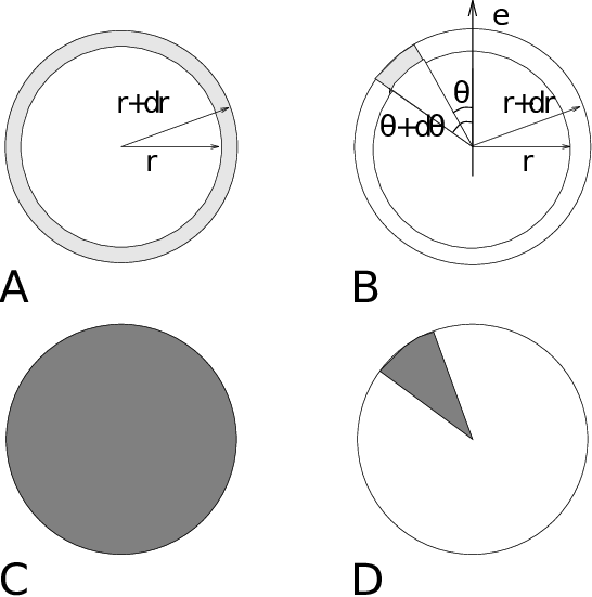
Fig. 51 Definition of slices in gmx rdf: A. \(g_{AB}(r)\). B. \(g_{AB}(r,\theta)\). The slices are colored gray. C. Normalization \(\langle\rho_B\rangle_{local}\). D. Normalization \(\langle\rho_B\rangle_{local,\:\theta }\). Normalization volumes are colored gray.

Usually the value of \(r_{max}\) is half of the box length. The averaging is also performed in time. In practice the analysis program gmx rdf divides the system into spherical slices (from \(r\) to \(r+dr\), see Fig. 51 A) and makes a histogram in stead of the \(\delta\)-function. An example of the RDF of oxygen-oxygen in SPC water :ref:80 is given in Fig. 52

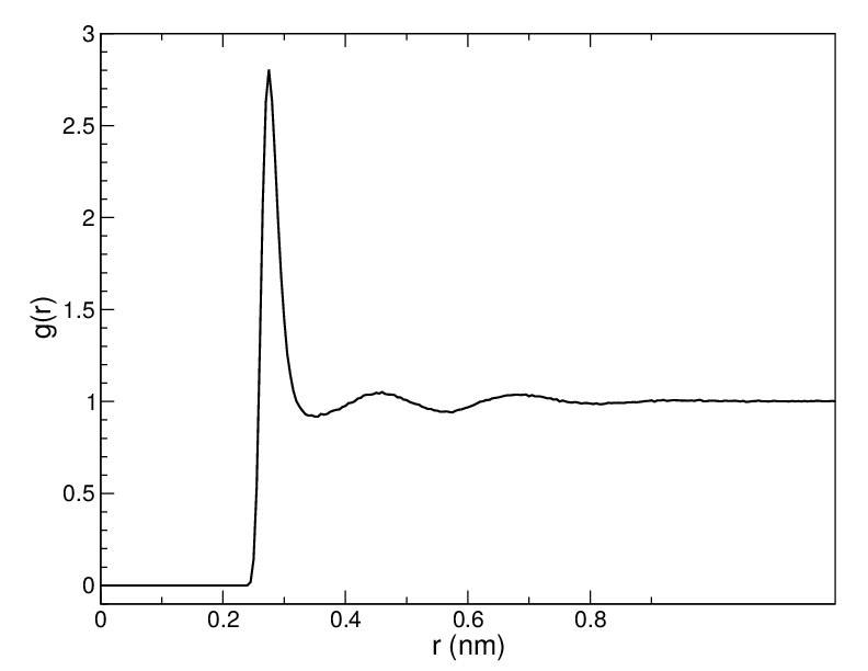
Fig. 52 \(g_{OO}(r)\) for Oxygen-Oxygen of SPC-water.

With gmx rdf it is also possible to calculate an angle dependent rdf \(g_{AB}(r,\theta)\), where the angle \(\theta\) is defined with respect to a certain laboratory axis \({\bf e}\), see Fig. 51 B.

(2)\[g_{AB}(r,\theta) = {1 \over \langle\rho_B\rangle_{local,\:\theta }} {1 \over N_A} \sum_{i \in A}^{N_A} \sum_{j \in B}^{N_B} {\delta( r_{ij} - r ) \delta(\theta_{ij} -\theta) \over 2 \pi r^2 sin(\theta)}\]

(3)\[cos(\theta_{ij}) = {{\bf r}_{ij} \cdot {\bf e} \over \|r_{ij}\| \;\| e\| }\]

This \(g_{AB}(r,\theta)\) is useful for analyzing anisotropic systems. Note that in this case the normalization \(\langle\rho_B\rangle_{local,\:\theta}\) is the average density in all angle slices from \(\theta\) to \(\theta + d\theta\) up to \(r_{max}\), so angle dependent, see Fig. 51 D.